발틱운임지수(BDI)와 해양운송업
발틱운임지수(BDI)와 해양운송업(팬오션, 대한해운)
해양운송업은 발틱운임지수(BDI)와 밀접한 관련이 있다. pandas_datareader을 사용하여 해양운송업의 두 종목의 가격과 BDI 데이터를 가져와 차트로 확인하고 상관계수도 구해본다.
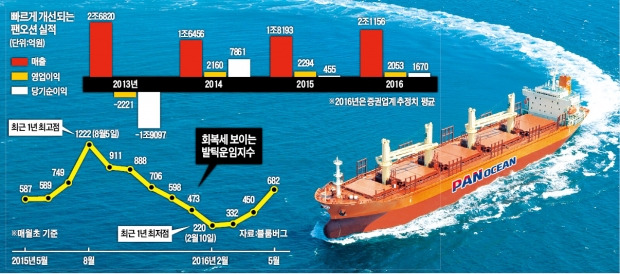 이미지출처: (한국경제) https://goo.gl/iFgU4m
2017 http://financedata.kr
In [1]:
%matplotlib inline
import matplotlib.pyplot as plt

plt.rcParams["axes.grid"] = True
plt.rcParams["figure.figsize"] = (14,4)
BDI, Baltic Dry Index
- BDI (Baltic Dry Index): 발틱 건화물(乾貨物) 운임 지수
- 1985년 1월 4일의 운임을 1000으로 볼 때 운임이 얼마나 내리고 올랐는지를 수치화한 것
- 벌크업황을 나타내는 대표적인 지표
데이터는 quandl 에서 구할 수 있다
BDI 데이터 가져오기
pandas_datareader를 사용하여, 2010년 1월 부터 현재까지 BDI를 간편하게 가져올 수 있다
In [2]:
import pandas_datareader as pdr

# 2010년 1월 부터 현재까지 BDI
df_bdi = pdr.DataReader('LLOYDS/BDI', 'quandl')
df_bdi.head()
Out[2]:
In [3]:
# 날짜 역순으로 되어 있어 인덱스인 'Data'로 소트
df_bdi.sort_index(inplace=True)
df_bdi.head()
Out[3]:
In [4]:
# 2016년 이후 BDI
df_bdi['2016':].plot()
Out[4]:

팬오션 주가
In [5]:
# 팬오션
df_pan = pdr.DataReader('028670.KS', 'yahoo')
df_pan.head()
Out[5]:
BDI지수 + 팬오션 주가
In [6]:
import pandas as pd

df = pd.DataFrame() # 빈 DataFrame 생성
df['BDI'] = df_bdi['Index']
df['Pan Ocean'] = df_pan['Adj Close']
df.sort_index(inplace=True)
In [7]:
df.plot(secondary_y='BDI')
Out[7]:

BDI 와 팬오션(Pan Ocean)의 수정종가사이의 상관계수를 구해본다. 0.74 상당히 높게 나온다.
In [8]:
df.corr()
Out[8]:
In [9]:
# 2015년 이후만 따로 뽑아 본다

df_2015 = df['2015':]
df_2015.plot(secondary_y='BDI')
Out[9]:

In [10]:
df_2015.corr() # 0.737 상당히 높게 나온다
Out[10]:
대한해운에 대해 동일한 분석
대한해운(005880)에 대해 동일한 비교 분석을 해본다
In [11]:
df_koline = pdr.DataReader('005880.KS', 'yahoo')
df_bdi = pdr.DataReader('LLOYDS/BDI', 'quandl')

df = pd.DataFrame() # 빈 DataFrame 생성
df['BDI'] = df_bdi['Index']
df['KoLine'] = df_koline['Adj Close']
df.sort_index(inplace=True)

df.plot(secondary_y='BDI')
Out[11]:

In [12]:
df.corr()
Out[12]:
In [13]:
# 2016년 이후만 그려본다

df['2016':].plot(secondary_y='BDI')
Out[13]:

참고자료
- https://goo.gl/Kogdq5 돈이 보이는 경제 지표 - 발틱운임지수(BDI) -- 중앙일보
- https://goo.gl/iFgU4m 2016-05-09 팬오션의 이유있는 순항 -- 한국경제
- https://goo.gl/9j3kTx 2017-07-20 "팬오션, 건화물선 운임지수(BDI) 개선되며 이익증가도 기대" - KB
- https://goo.gl/a4ypm3 2017-01-02 [Top-Down] BDI 지수와 해운산업, 대학원생 '옹쿠'의 공부하는 블로그
댓글
Comments powered by Disqus